Chirun: A Reference Guide for Users

Ross Parker

April 2025

1 Introduction

This documents acts as a template and reference guide for using the L^aT_eX to HTML conversion tool Chirun ( Chirun Project 2025a ) . This document is built from a tex file, and converted to HTML. Chirun also supports the conversion of markdown md files to HTML.

When uploading existing L^aT_eX notes for the first time, there’s a good chance Chirun will fail to convert them to HTML and you’ll see a long console log containing various errors. This can be very frustrating and you may be tempted to give up, and stick with using PDF documents. Bear with it though, as the benefits of using Chirun are worth it.

Using Chirun, you can create HTML documents that are accessible to screen readers and other assistive technologies, and you can also embed videos and images in your documents. This is a great way to make your notes more engaging and interactive for your students.

If you use this document to better understand which L^aT_eX packages Chirun supports ( Chirun Project 2025b ) , and how best to format your L^aT_eX documents, you can create accessible L^aT_eX HTML documents ( World Wide Web Consortium (W3C) 2023 ) .

While HTML is the gold standard for accessibility, Chirun also generates a PDF version of your notes that can be particularly useful for students who like to annotate their notes. Try clicking the Download as PDF link above the Table of Contents.

2 Including Images

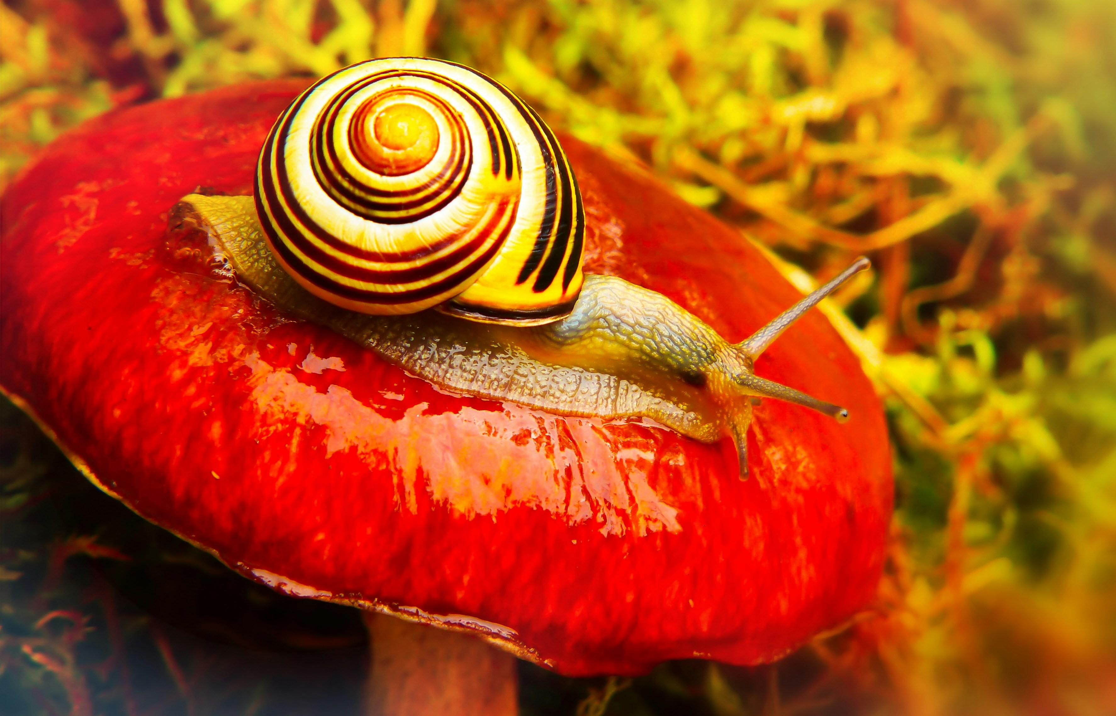
The insertion of images makes use of the \chirun package, by allowing alternative text to be inserted using the \alttext command. If you use assisitive technologies such as a screenreader, this image will be read out as follows: ’A snail with a yellow and brown spiral patterned shell on the top of a red mushroom.’ Without the \alttext command, the screenreader would read out the file name of the image instead, which is not very helpful and will unfairly disadvantage anyone with a visual impairment.

A snail with a yellow and brown spiral patterned shell on the top of a red mushroom. — Figure 1 A spiral formed by Fibonacci-numbered squares resembles a snail shell—an elegant pattern often used in art and design. Photo by Krzysztof Niewolnyn on Unsplash

3 Quotations

You can make quotations stand out by using the \quote or \quotation command. If you want to add coloured boxes for things like derivatives or theorems, see the section on using coloured boxes.

“The Fibonacci Sequence turns out to be the key to understanding how nature designs... and is... a part of the same ubiquitous music of the spheres that builds harmony into atoms, molecules, crystals, shells, suns and galaxies and makes the Universe sing.”

Guy Murchie

4 Making Lists

Here are examples of creating lists. The first is an ordered list using {enumerate} and the second is an unordered list using {itemize}.

4.1 Ordered Lists

This photography workflow outlines the key steps a photographer follows, from capturing an image to producing the final output. Each stage builds upon the previous one, demonstrating a clear, sequential process.

Shoot – Capture the image using the best settings for your scene and creative intent.
Transfer – Move the photos from your camera to your computer or cloud storage for backup.
Edit – Adjust exposure, color balance, cropping, and apply creative edits to enhance the image.
Publish – Share the edited image online, whether on social media, websites, or portfolios.
Print – Create physical copies for display, framing, or professional use.

4.2 Unordered Lists

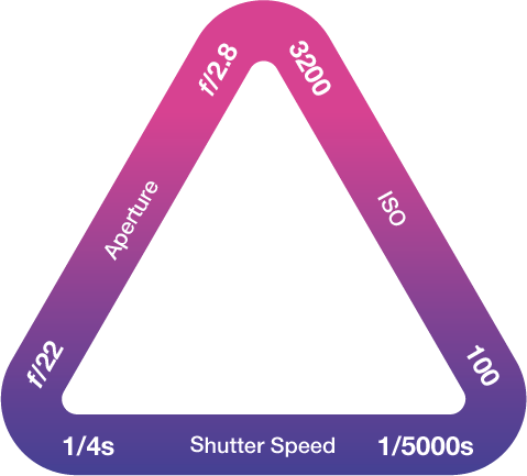
Capturing light for image rendition requires a basic understanding of the fundamentals of the exposure triangle, which is composed of three parameters:

Aperture – Controls the size of the lens opening, affecting depth of field.
Shutter Speed – Determines how long light is exposed to the sensor, influencing motion blur.
ISO – Adjusts sensor sensitivity to light, balancing exposure and noise levels.

5 Maths Equations

When converting LaTeX documents to HTML, mathematical notation is often rendered using MathJax. This ensures that equations are displayed clearly in web browsers and remain accessible to screen readers and other assistive technologies.

5.1 The Fibonacci Sequence

The Fibonacci sequence ( of Pisa 1202 ) is a famous number pattern where each number is the sum of the two before it. It begins like this:

\[ 0,\ 1,\ 1,\ 2,\ 3,\ 5,\ 8,\ 13,\ 21,\ 34,\ \dots \]

5.2 Recursive Definition

The Fibonacci sequence can be defined using a simple recursive formula:

$\begin{equation}F_0 = 0,\quad F_1 = 1,\quad F_n = F_{n-1} + F_{n-2} \quad \text{for } n \geq 2\tag{1}\end{equation}$

5.3 Closed-form Formula (Binet’s Formula)

We can also calculate the $n$th Fibonacci number directly using a closed-form formula, though it’s a bit more complex:

$\begin{equation}F_n = \frac{1}{\sqrt{5}} \left( \phi ^n - \left( -\frac{1}{\phi } \right)^n \right)\tag{2}\end{equation}$

where $\phi $ (phi) is the golden ratio:

$\begin{equation}\phi = \frac{1 + \sqrt{5}}{2}\tag{3}\end{equation}$

5.4 The Golden Ratio

As the sequence continues, the ratio between consecutive Fibonacci numbers approaches the golden ratio:

$\begin{equation}\lim _{n \to \infty } \frac{F_{n+1}}{F_n} = \phi \approx 1.618\tag{4}\end{equation}$

This ratio appears in many areas of nature, design, and photography.

5.5 Matrix Representation

Fibonacci numbers can even be represented using matrices, which is useful for advanced calculations:

$\begin{equation}\begin{bmatrix} F_{n+1} \\ F_n \end{bmatrix} = \begin{bmatrix} 1 & 1 \\ 1 & 0 \end{bmatrix}^n \begin{bmatrix} 1 \\ 0 \end{bmatrix}\tag{5}\end{equation}$

This shows that the Fibonacci sequence has many layers, from simple patterns to deeper mathematical structures.

6 Using Tables

Tables can be useful for presenting sets of related data at a glance. In photography, the exposure triangle is often represented through typical values for aperture, shutter speed, and ISO ( Mansurov 2024 ) .

Aperture (f-stop)	Shutter Speed	ISO
f/1.4	1/1000 sec	100
f/2.8	1/500 sec	200
f/4	1/250 sec	400
f/5.6	1/125 sec	800
f/8	1/60 sec	1600
f/11	1/30 sec	3200
f/16	1/15 sec	6400

Table 1 Typical Exposure Triangle Settings

Note: The values in each row are illustrative and may not correspond to correct exposure in real-life scenarios. The appropriate settings depend on the amount of available light. For example, choosing f/4 and ISO 400 may require a different shutter speed than 1/250th second to achieve proper exposure.

Figure 2 An illustration of the exposure triangle, showing the relationship between aperture, shutter speed, and ISO.

7 Coloured Boxes

Shaded boxes are supported using the tcolorbox package. The colours are applied using the [dvipsnames] option within the xcolor package.

7.1 A Theorem in a Blue Box

Let $ f $ be a continuous function on a closed interval $[a, b]$. Then $ f $ is bounded on $[a, b]$, and there exist points $ c, d \in [a, b] $ such that: \[ f(c) \leq f(x) \leq f(d) \quad \text{for all } x \in [a, b]. \]

7.2 An Example in a Yellow Box with a Heading Section

Example

Consider the function $ f(x) = \sin x $ on the interval $[0, \pi ]$. Since sine is continuous on this interval, it is bounded. In fact, \[ \min _{x \in [0, \pi ]} \sin x = 0 \quad \text{and} \quad \max _{x \in [0, \pi ]} \sin x = 1. \]

8 Code Highlighting Using the Listings Package

Code can be highlighted using the listings package. The following example shows how to create a function that computes the incidence matrix of two generators. The function incmatrix takes two lists of generators as input and returns the incidence matrix. The code is written in Python and uses NumPy for matrix operations.

Listing 0.1: Python example

import numpy as np
    
def incmatrix(genl1,genl2):
    m = len(genl1)
    n = len(genl2)
    M = None #to become the incidence matrix
    VT = np.zeros((n*m,1), int)  #dummy variable
    
    #compute the bitwise xor matrix
    M1 = bitxormatrix(genl1)
    M2 = np.triu(bitxormatrix(genl2),1) 

    for i in range(m-1):
        for j in range(i+1, m):
            [r,c] = np.where(M2 == M1[i,j])
            for k in range(len(r)):
                VT[(i)*n + r[k]] = 1;
                VT[(i)*n + c[k]] = 1;
                VT[(j)*n + r[k]] = 1;
                VT[(j)*n + c[k]] = 1;
                
                if M is None:
                    M = np.copy(VT)
                else:
                    M = np.concatenate((M, VT), 1)
                
                VT = np.zeros((n*m,1), int)
    
    return M

9 Including Videos

Videos can be embedded from YouTube or Vimeo so they appear in the HTML output. They are rendered as hyperlinks in the PDF output. For more information visit the Chirun LaTeX package documentation ( Graham 2022 ) .

10 Scientific Charts and Diagrams

10.1 Plotting Mathematical Expressions Using a Line Graph

$\begin{tikzpicture} \begin{axis}[ width=12cm, height=8cm, % Increased size axis lines = left, xlabel = $x$, ylabel = {$f(x)$}, ] % Below the red parabola is defined \addplot [ domain=-10:10, samples=100, color=red, ] {x^2 - 2*x - 1}; \addlegendentry{$x^2 - 2x - 1$} % Here the blue parabola is defined \addplot [ domain=-10:10, samples=100, color=blue, ] {x^2 + 2*x + 1}; \addlegendentry{$x^2 + 2x + 1$} \end{axis} \end{tikzpicture}$

10.2 Plotting Mathematical Expressions Using the Mesh Parameter

$\begin{tikzpicture} \begin{axis}[ width=12cm, height=8cm, % Increased size title=Example using the mesh parameter, hide axis, colormap/cool, ] \addplot3[ mesh, samples=50, domain=-8:8, ] {sin(deg(sqrt(x^2+y^2)))/sqrt(x^2+y^2)}; \addlegendentry{$\frac{\sin(r)}{r}$} \end{axis} \end{tikzpicture}$

References

[1]

Chirun Project 2025a, Chirun Sample Course, Chirun Project. https://chirun-ncl.github.io/sample_course/.
[2]

Chirun Project 2025b, Chirun Tutorial, Chirun Project. https://chirun.org.uk/docs/en/latest/getting_started/tutorial.html.
[3]

Graham, C. 2022, ‘Building accessible, enriched learning materials with chirun’, https://www.youtube.com/watch?v=BAIAlWS3FRE. Presented by Dr. Chris Graham on the Maths Support Centre YouTube channel.
[4]

Mansurov, N. 2024, ‘Understanding iso, shutter speed and aperture – a beginner’s guide’. Accessed: 2025-05-12.
https://photographylife.com/iso-shutter-speed-and-aperture-for-beginners
[5]

of Pisa, L. 1202, Liber Abaci, Unknown. Introduced the Fibonacci sequence to Western mathematics.
[6]

World Wide Web Consortium (W3C) 2023, ‘Web content accessibility guidelines (wcag) 2.2’, https://www.w3.org/TR/WCAG22/. Accessed: 2025-05-12.

Test Yourself